Antenna plotting program for plotting antenna simulation results
Project description
This is a program to plot antenna-related data resulting from an antenna simulation. It can read the text output produced by nec2c and my python mininec port pymininec. Most notably it can plot antenna far-field pattern in both 2D (Azimuth and Elevation) and 3D (as a 3D graphic that can be rotated and zoomed). It supports a local display program (using matplotlib) and a HTML output version that displays everything using javascript (using plotly). The program features a --help option. If the program called with --help does not display a -H or --export-html option, you most likely do not have a recent version of plotly installed. In that case only the matplotlib variant is available.
The program started out as a companion-program to my pymininec project and is now an independent program.
The plot program can also display output files of nec2c, not only from pymininec.
Standalone Plotting with Matplotlib
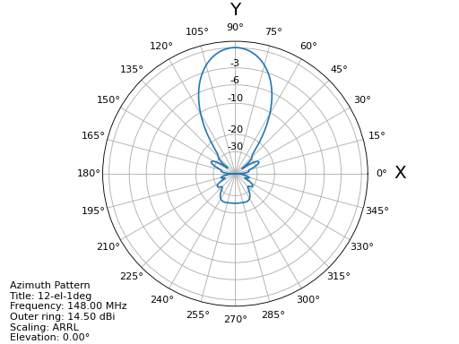
The default is to plot all available graphics, including an interactive 3d view. In addition with the --azimuth or --elevation options you can get an Azimuth diagram:
plot-antenna --azimuth test/12-el-1deg.pout

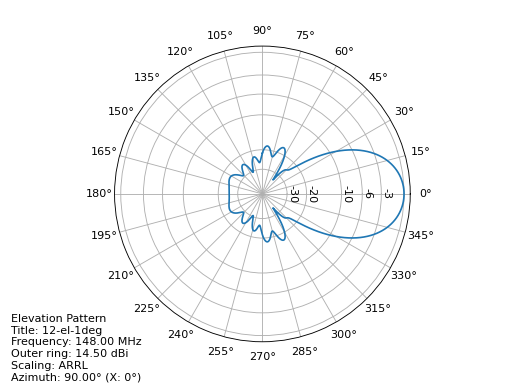
or an elevation diagram:
plot-antenna --elevation test/12-el-1deg.pout

respectively. Note that I used an output file with 1-degree resolution in elevation and azimuth angles not with 5 degrees as in the example above. The pattern look smoother but a 3D-view will be very slow due to the large number of points. The plot program also has a --help option for further information. In particular the scaling of the antenna plot can be selected using the --scaling-method option with an additional keyword which can be one of linear, linear_db, and linear_voltage in addition to the default of arrl scaling. You may consult Cebik’s [1] article for explanation of the different diagrams. The linear_voltage option is not explained by Cebik, it is in-between the linear and linear_db scaling options.
The latest version accepts several plot parameters, --elevation, --azimuth, --plot3d, --plot-vswr, and --geo which are plotted into one diagram. The default is to plot the first four graphs. With the --output option pictures can directly be saved without displaying the graphics on the screen. Note that unfortunately the geometry display with the --geo option does not perform very well because matplotlib has poor support for panning and scaling in 3D plots.
The latest version has key-bindings for scrolling through the frequencies of an antenna simulation. So if you have an output file with a simulation of multiple frequencies (either with pymininec or nec2c) you can display diagrams for the next frequency by typing +, and to the previous frequency by typing -. For newer versions of matplotlib you can display a scrollbar for the frequencies with the --with-slider option.
Other keybindings switch the scaling for the antenna plots, a switches to arrl scaling, l switches to linear scaling, d switches to linear dB scaling, and v switches to linear voltage scaling.
Finally the w key toggles display of the 3d diagram from/to wireframe display. Note that the wireframe display may not be supported on all versions of matplotlib and/or graphics cards.
Plotting for the Browser with Plotly
All the plot supported for matplotlib are also supported with plotly. These are --elevation, --azimuth, --plot3d, --plot-vswr, and --geo. The plots can be either exported to a .html file using the -H or --export-html option (with an additional filename to export to) or injected into a running browser using the -S or --show-in-browser option.
Unlike for matplotlib, each plot selected with an option is either shown in a separate window in the browser or exported to a separate file. If exporting to a file, additional output options can be selected with the --html-export-option setting. The default is to export the file with all javascript included (adds about 3MB to the file size). With --html-export-option=directory the javascript is not included and a plotly.min.js file is expected in the same directory as the exported file. This file ships with the plotly distribution. When exporting to a file, the plot name is appended to the file name given, this allows export to several different plots in one program invocation.
The scaling variants selected with the --scaling-method option cannot currently be changed at runtime with the plotly plots. As with matplotlib, the default is arrl scaling.
All plots are interactive. For the far-field pattern plots (Azimuth, Elevation, 3D) frequencies can be selected in the legend to the right of the plot. With mouse-over you can see the current angle (Elevation or Azimuth with the 2D plots and both for the 3D plot) and the gain at that point. For the 2D variants, more than one frequency can be selected for plotting. This allows comparison of pattern between different frequencies. For the 3D plot, the frequencies in the legend act like radio-buttons, only one at a time can be selected.
With the –geo option you get a display of the antenna geometry. Unfortunately plotly seems to have limitations on the zoom depths, so for large antennas it is not possible to see the plot in deep detail. As of this writing not all geometry details are displayed. In particular 2D patches in NEC, transmission lines in NEC, and visualization of loaded segments (e.g. with a capacity) are not shown.
Project details
Download files
Download the file for your platform. If you're not sure which to choose, learn more about installing packages.
Source Distribution
File details
Details for the file plot-antenna-1.0.tar.gz.
File metadata
- Download URL: plot-antenna-1.0.tar.gz
- Upload date:
- Size: 21.4 kB
- Tags: Source
- Uploaded using Trusted Publishing? No
- Uploaded via: twine/4.0.1 CPython/3.9.2
File hashes
| Algorithm | Hash digest | |
|---|---|---|
| SHA256 | 883bd2f9088a527f4e70174b0cab771ef6c00dd1aa6f098b03354cb7cd1670f4 |
|
| MD5 | dd22035f08e4a74093a2131250bacc4b |
|
| BLAKE2b-256 | 03219ec64d883c732907d1e26aeb6cf2b5af2352378676dc9ee7cdf05ed05498 |


